
In this tutorial you will convert a digital elevation model (DEM) along a river of your choice into a relative elevation model (REM) in QGIS using the cross-section method. If you haven't tried the Creating REMs in QGIS using the IDW Method tutorial yet, I encourage you to start with those methods first, since they are generally faster and easier to replicate.
The example dataset is a bare-earth lidar DEM (aka digital terrain model or DTM) along the Carson River in western Nevada.
The tutorial is geared toward users who have some experience using GIS and have QGIS installed on their computer. Users will also need a DEM along a river of their choice to get started (go here if you need a DEM). This tutorial will likely take approximately 3 hours to complete, but the time may differ depending on the length of your river and processing time.
This tutorial can be done independently or in combination with the: Downloading and Preparing Lidar DEMs for REM Processing tutorial and the Exporting Images from QGIS tutorial.
REMs, an Introduction
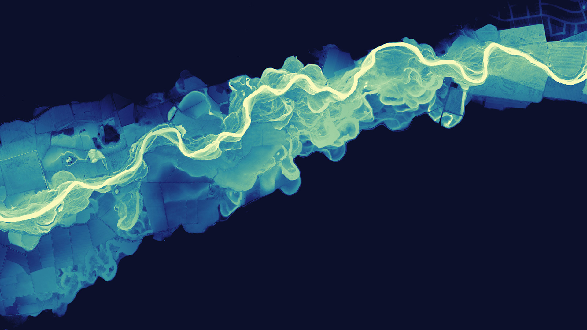
In floodplains, lidar digital elevation models (DEMs) can be converted to relative elevation models (REMs) to better visualize river features that are difficult to discern using an aerial photo or standard DEM. REMs, also know as height above river (HAR) rasters, are produced by detrending the baseline elevation to follow the water surface of the stream. In a DEM, the baseline elevation (0 feet or meters) is at sea level and the downstream part of a river has a lower elevation than the upstream part. In a REM, the baseline elevation (0 feet or meters) is detrended to follow the water surface of a river—elevations trend higher as one moves away from the river, showing the "relative" height above river.
REMs are extremely useful in discerning where river channels have migrated in the past by vividly displaying river features such as meander scars, terraces, and oxbow lakes. This type of information is very informative in channel migration and flood studies, as well as a host of other engineering, habitat, and cultural assessments.
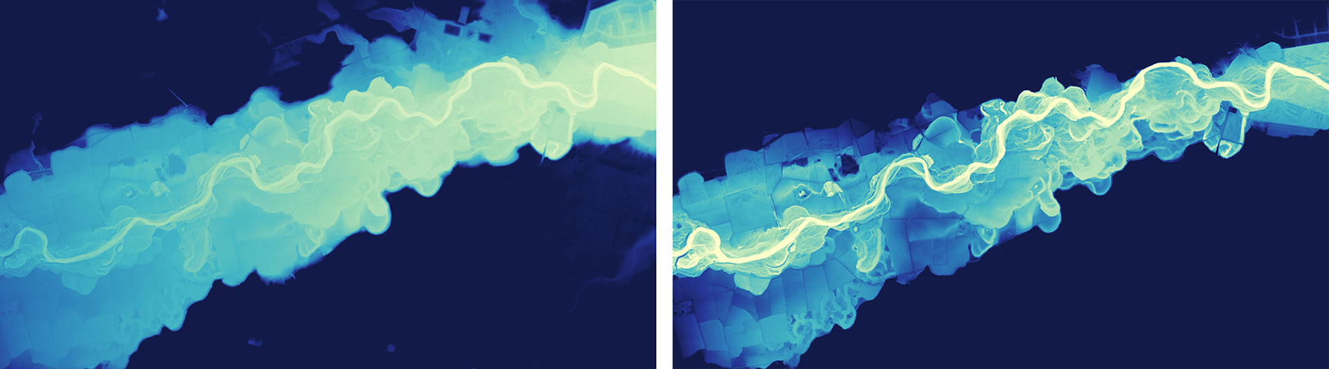
Left: A digital elevation model of the Carson River with the baseline elevation (0) at sea level. Right: A relative elevation model (REM) of the same area with the baseline elevation (0) at the water surface of the river.
Another reason I personally make REMs of rivers, however, is that they are intrinsically beautiful. Many REMs translate into wonderful flowing artistic images that are a visual time capsule of a river's natural history. They are a subject that satisfies both a scientific and aesthetic curiosity about the world.
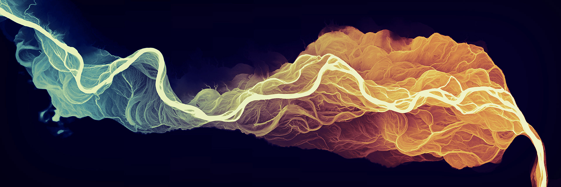
Relative elevation model of the Snake River in Grand Teton National Park, Wyoming.
REMs can be created using a number of different methods. I have written QGIS methods for two techniques, the IDW method (the previous tutorial) and the Cross-Section method (this tutorial). These methods were adapted from the ArcGIS Desktop steps described by Olson and others (2014). These techniques use point (IDW) and line (cross-section) GIS data that possess elevations corresponding to the river's surface. These data are interpolated to create a new raster surface and then subtracted from the original DEM raster to create the REM.
Occasionally, more than one iteration of the model is needed to accurately represent the water surface at 0 elevation. Some common factors and features that reduce model accuracy are: rivers with a steep elevation gradient, rivers with high sinuosity, dams, steep waterfalls, tidal areas, braided channels, and mosaicked datasets from different time periods.
Large, slow moving, meandering rivers represented with high-resolution lidar DEMs work best for these techniques, but don't let that stop you if your river and dataset don't fit these criteria. I have seen very interesting results from an array of river types and raster resolutions.
If you have a single DEM that is ready to go you can dive right in to this tutorial. If you are looking for a dataset I encourage you to use the Downloading and Preparing Lidar DEMs for REM Processing tutorial to get started.
These are some of the first tutorials that I have written so I welcome any feedback that will make them better. As with all things GIS, there are multiple ways to do things, so if there are more efficient steps that will improve the methods described here please let me know! I hope to add a video version of this tutorial (and the others) in the future and the feedback will make those efforts easier.
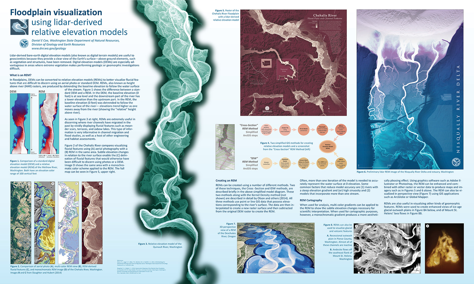
For more information on REMs click on the poster below.
Creating the REM
A. Create a project folder and put your river DEM there.
Open QGIS, then save the QGIS project to your project folder.
For this tutorial I used QGIS 3.16 Hannover Long Term Release, but the steps should be the same for all recent releases.
Remember to save your project periodically throughout this tutorial so you don't lose your work!
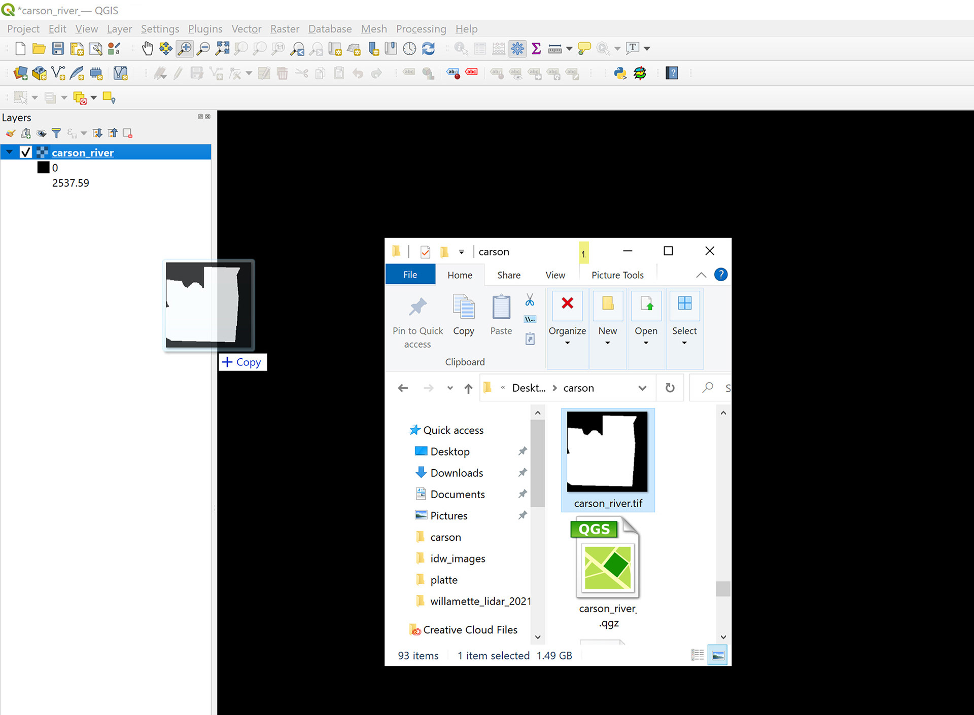
Once QGIS is open, drag your DEM (in this case, the carson_river.tif) into the Layers window, or load it with the Data Source Manager.
If you get a Select Transformation window when you add the data, select ok.
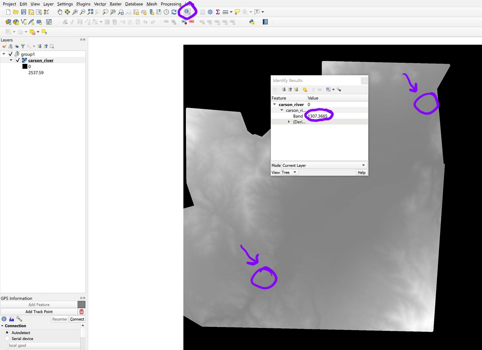
B. Select the Identify Features tool (see below).
With the tool selected click on the raster near the upstream and downstream end of your river to get the general elevation range (Band 1 in the results window shown below) along the river.
You might have to click around and explore a little to get the range.
Make a mental note of the high and low elevations (or write them down) that you find on the upstream and downstream ends of your study area.
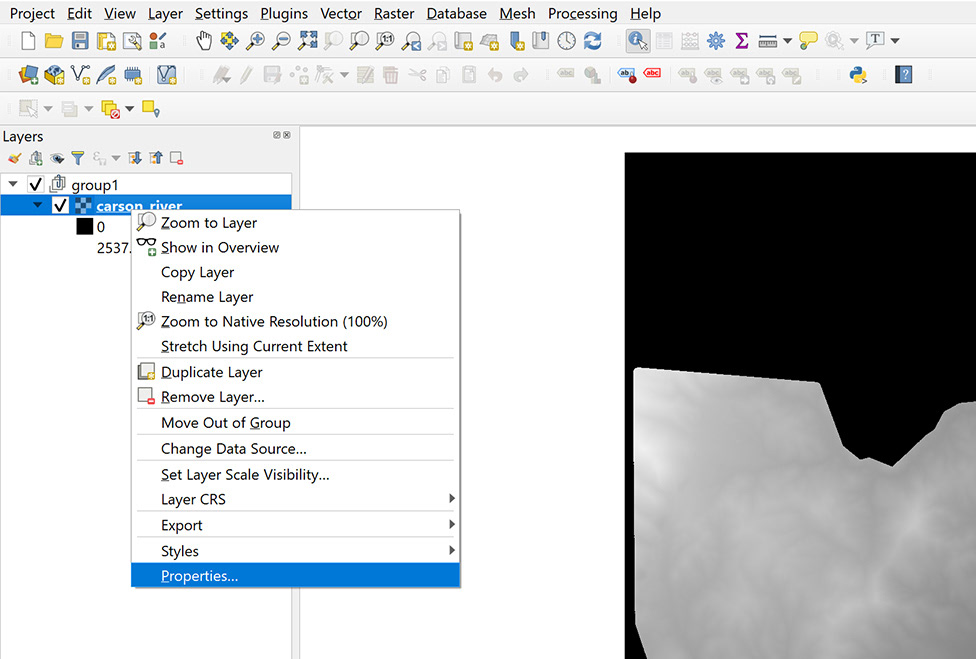
C. Right click on your DEM in the Layers window and select Properties.
D. In the Layer Properties window select Symbology in the panel on the left.
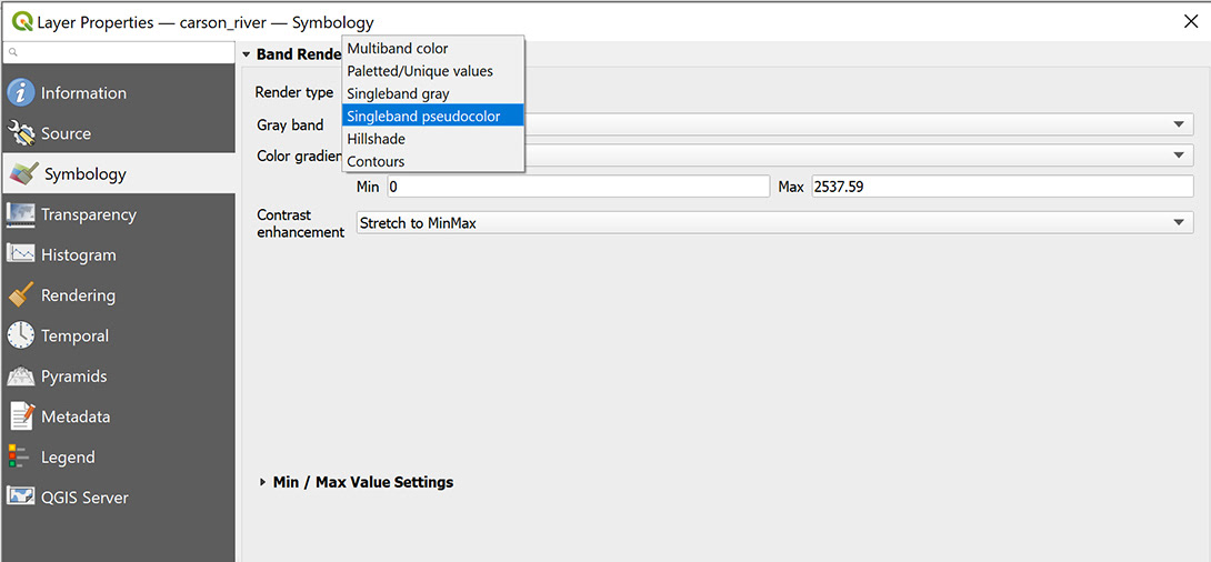
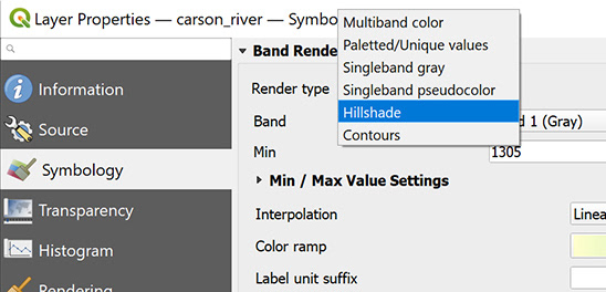
Select the Render type dropdown and select Singleband pseudocolor.
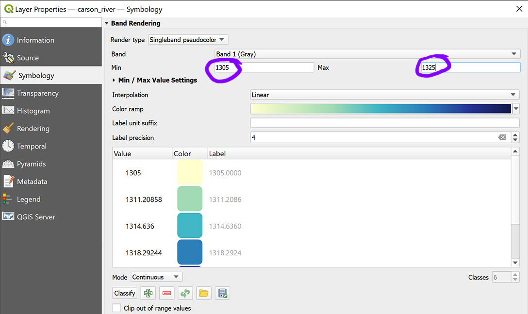
E. Enter the the low and high values of your sampled elevation ranges into the Min and Max boxes.
Select the Color ramp drop down and choose a color ramp that ranges from light to dark—preferably one that doesn't have too many jarring color changes.
Select Ok or Apply to apply the elevation and color changes to your DEM.
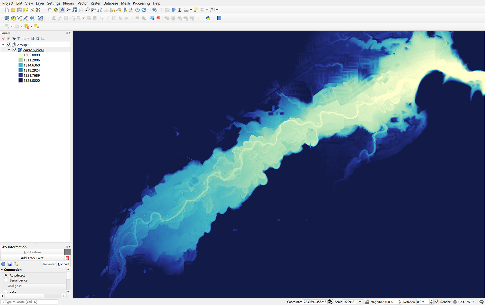
F. Take a look at your raster to make sure you can see the section of the river that you are interested in.
Adjust the Min/Max elevations in the Layer properties window as needed until you have a good range of color along the river (like the image below).
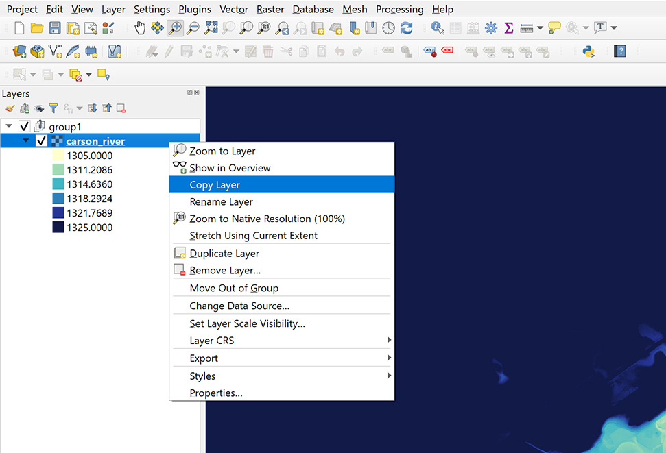
G. Make a copy of your DEM. Right click on the DEM in the Layers window and select Copy Layer.
Then right click in the Layers window and select Paste Layer/Group to paste the copied layer.
H. Right click on the top DEM layer in the Layers window and select Properties.
In the Layer Properties window Select the Render type drop down and choose Hillshade.
I. While still in the Layer Properties window, enter 5 in the Z Factor box to exaggerate the elevation for the hillshade (adjust this to your preference later if needed).
Under Color Rendering>Blending mode, select Soft Light.
Then select Ok at the bottom right.
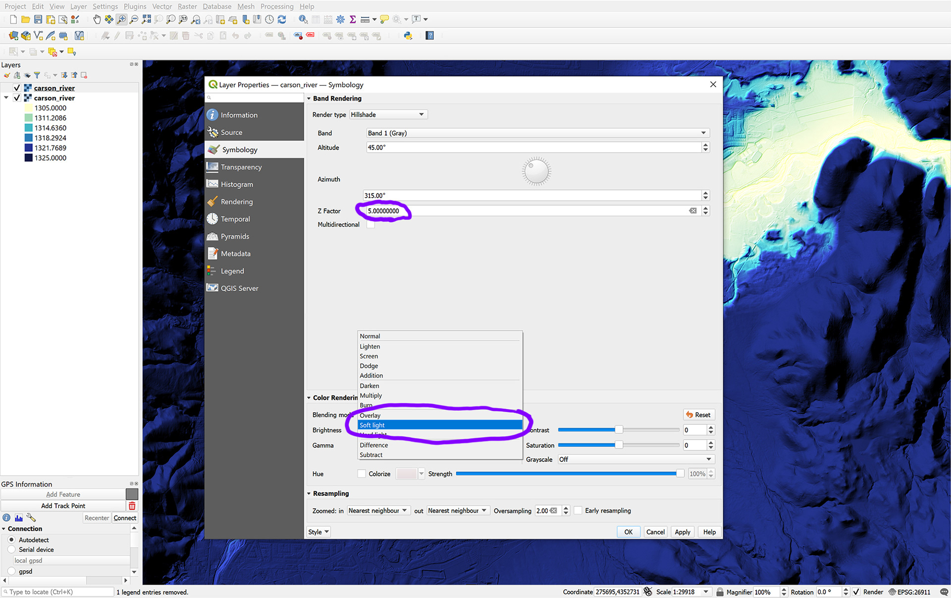
J. The exaggerated soft light hillshade should add a bit of definition to your DEM which will make the main river channel a little easier to see for the upcoming steps.

K. Create cross section file.
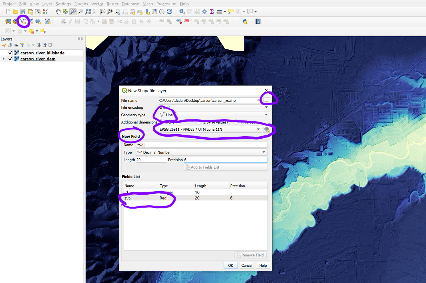
Add a line file type of your choice.
In this case I added a shapefile (shown below).
Select the file location and name (I usually name it something like river_name_xs).
For Geometry type select Line.
Check that the CRS is the same as your input file.
Under New field type zval for Name, Select Decimal Number for Type, then click on the Add to Fields List.
Select Ok.
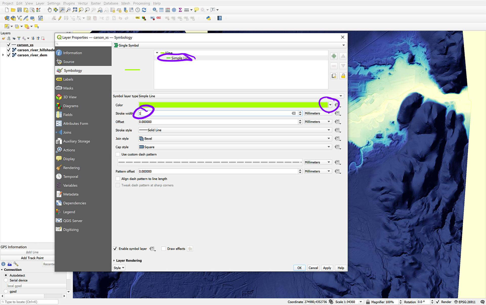
L. Go to Layer Properties>Symbology for your new line file.
Click on Simple line near the top and choose a bright color that you will be able to see against the background of your DEM.
Enter "1" in the stroke width box. Select Ok.
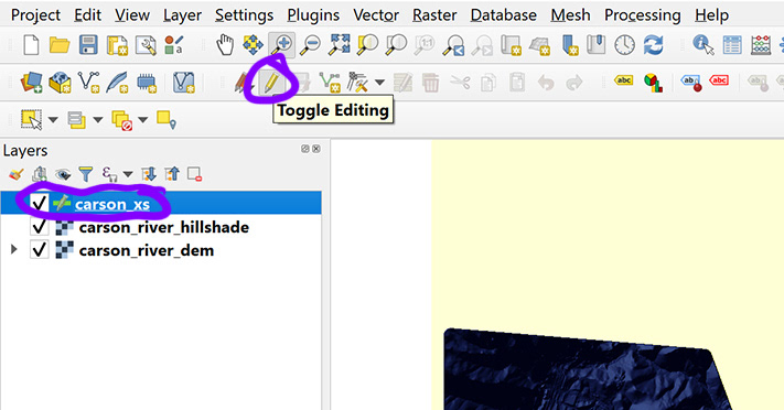
M. With your cross section line file selected in the Layer window, click on the Toggle Editing button to enable editing
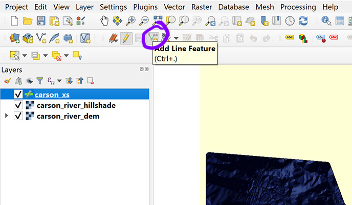
N. Select Add Line Feature in the tool bar (shown below).
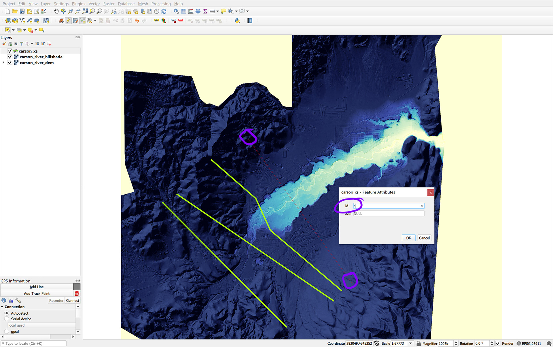
O. Create the cross section lines perpendicular to the river.
Make the lines long enough to cover the floodplain (or the area you want to include in the REM).
Click once to start the line, and so on to create more line nodes.
After you draw the last node, right click to end the line.
Add a ID number to the attribute box that appears when you finish the line.
You may have to angle segments of the lines to cross the river at a 90 degree angle (see cross section examples below).
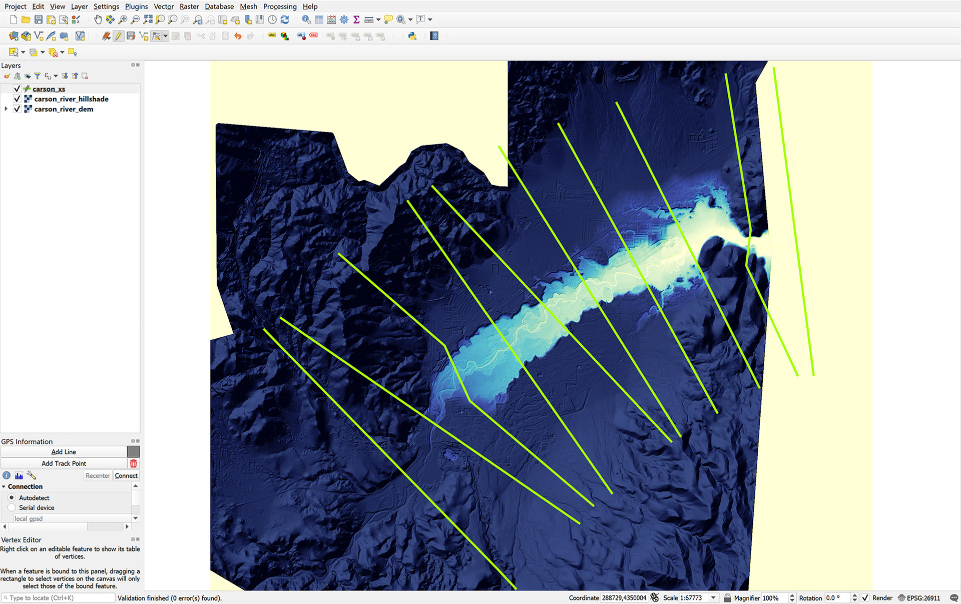
Create the lines at equally (or close to equally) spaced intervals along the river.
P. Draw cross sections across the entire length of the river in your study area.
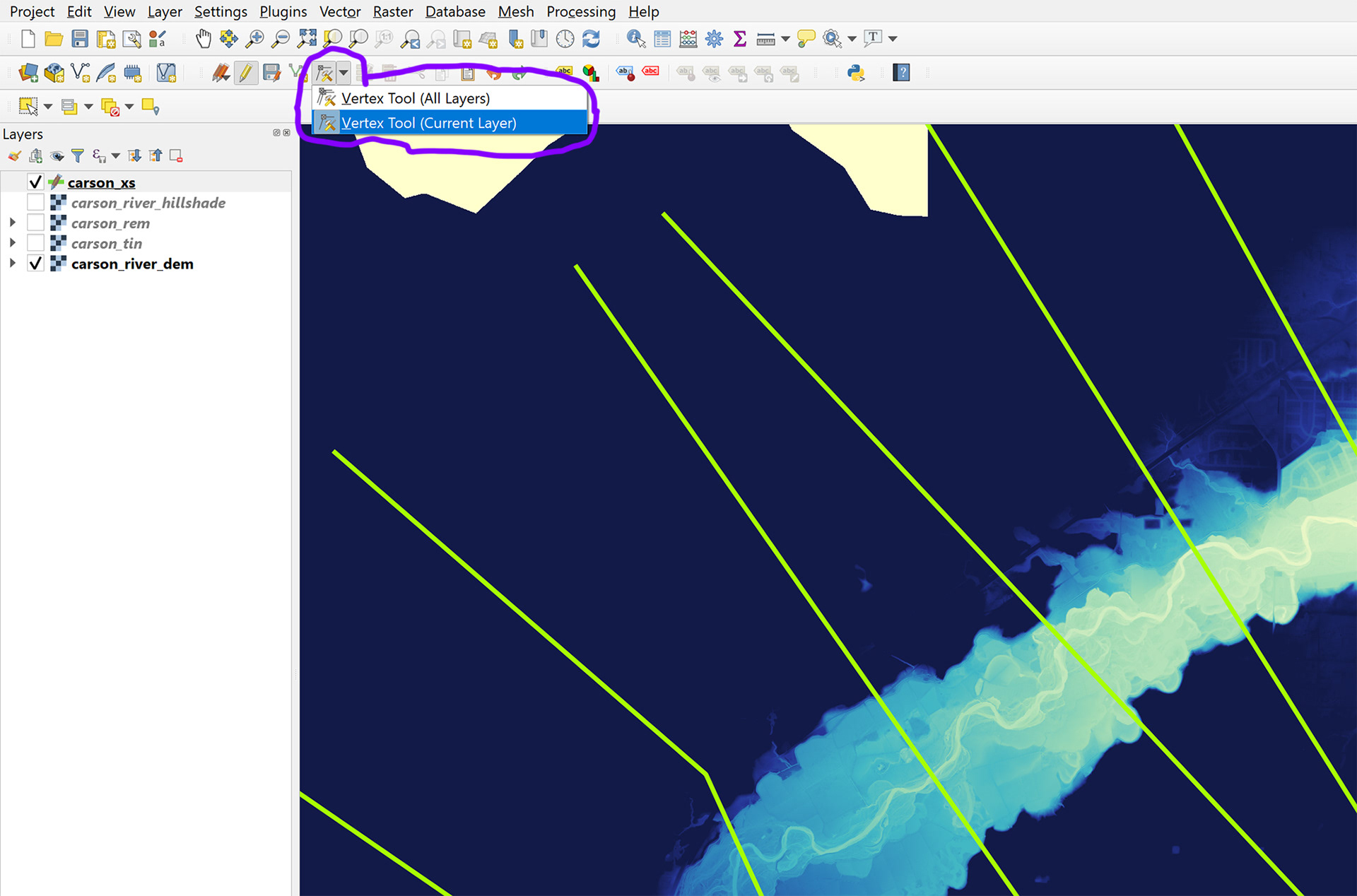
Q. If you need to edit any of the lines after you create them, use the Vertex Tool (shown below).
With the tool activated hover the cursor over a node or segment until it turns red, then click once to select.
After that you can move the node or segment to the desired location.
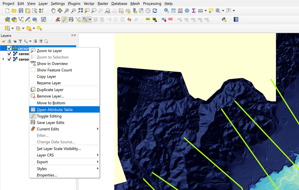
R. Once all of the cross section lines have been completed, right click on the cross section line layer and select Open Attribute Table.
In the attribute table, select the first row which will highlight the selected line in yellow on your screen.
Zoom into the area on your screen where the selected line crosses the river (see below).
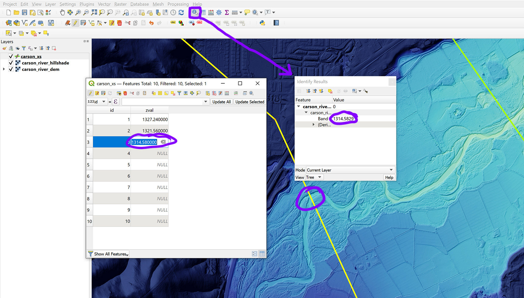
Using the Identify Features tool, right click on the river where the line intersects it, choose the DEM layer when the box appears.
In the Identify Results window find the elevation value (in this case, the value for Band 1) and enter that value into the zval attribute for the selected line in the attribute table.
With a river centerline file and a few extra steps this elevation extraction can be automated. However, in most cases it is faster to do this manually using the steps above.
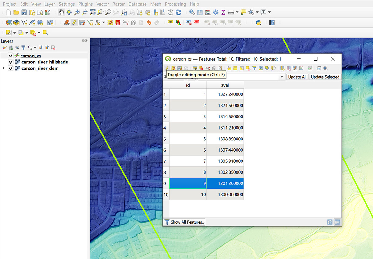
T. Enter elevation values for each of the cross section lines.
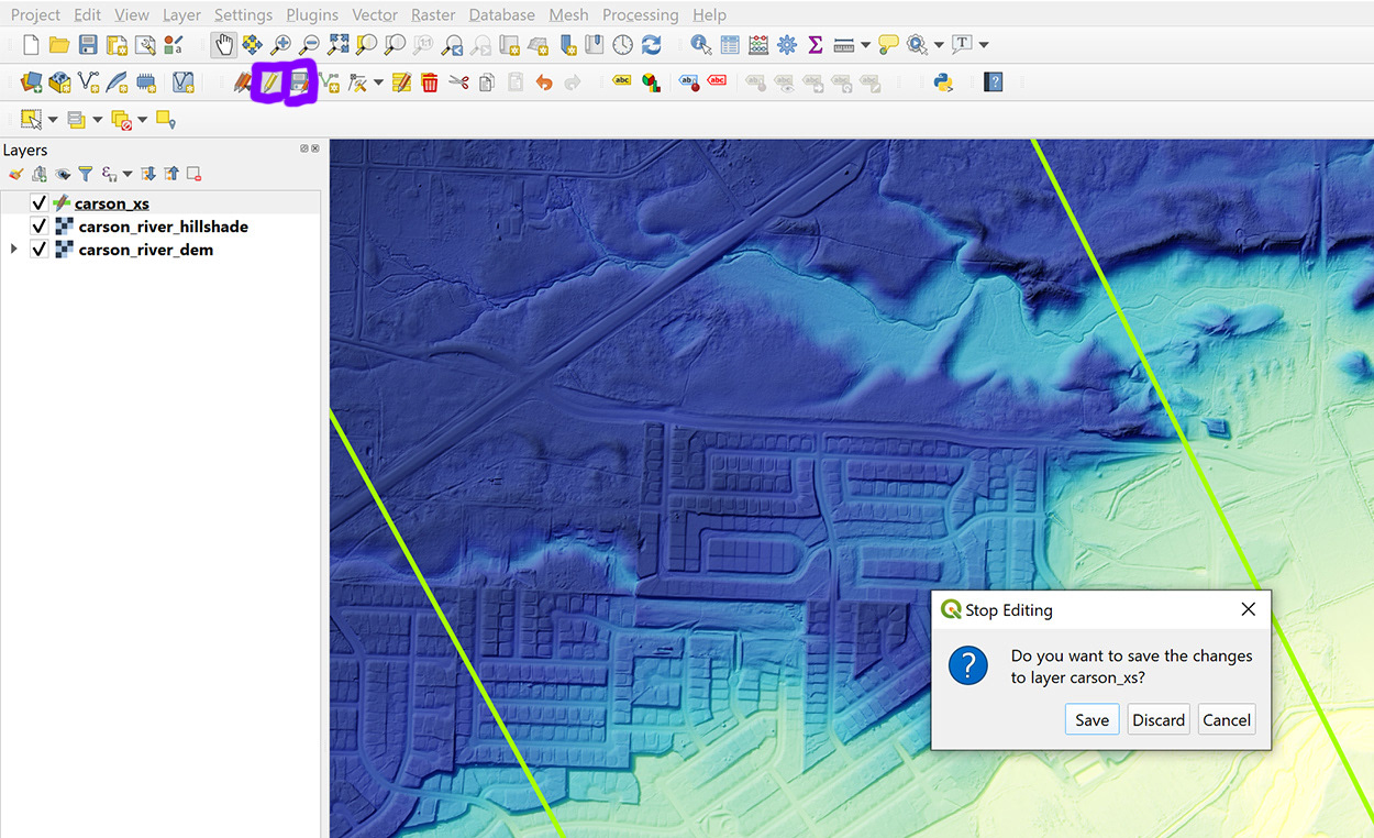
When they are all complete, click on the Toggle editing button to stop editing.
U. Be sure to select Save in the Stop Editing window (see below).
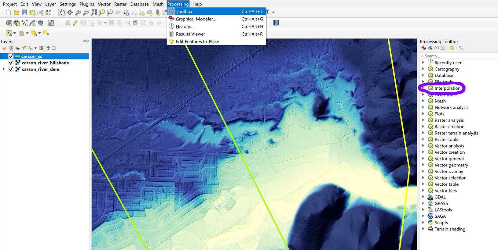
V. Go to Processing>Toolbox and select Interpolation in the Processing Toolbox that appears on the right side of the screen.
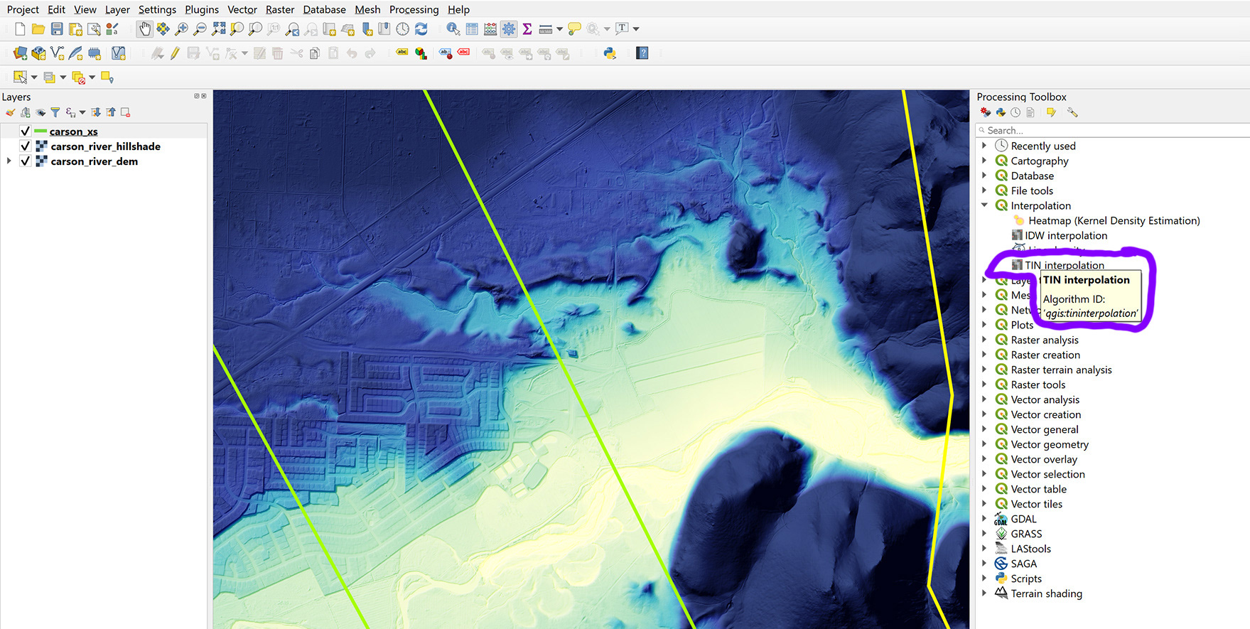
W. Under Interpolation select TIN Interpolation.
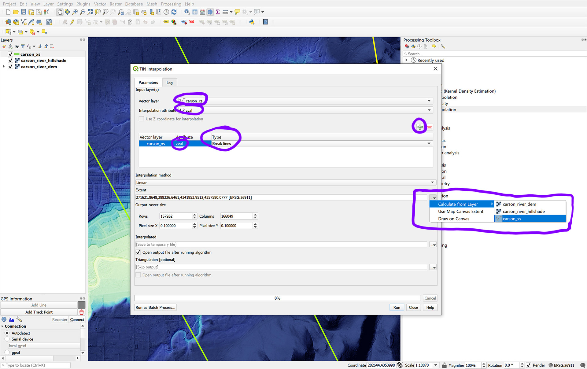
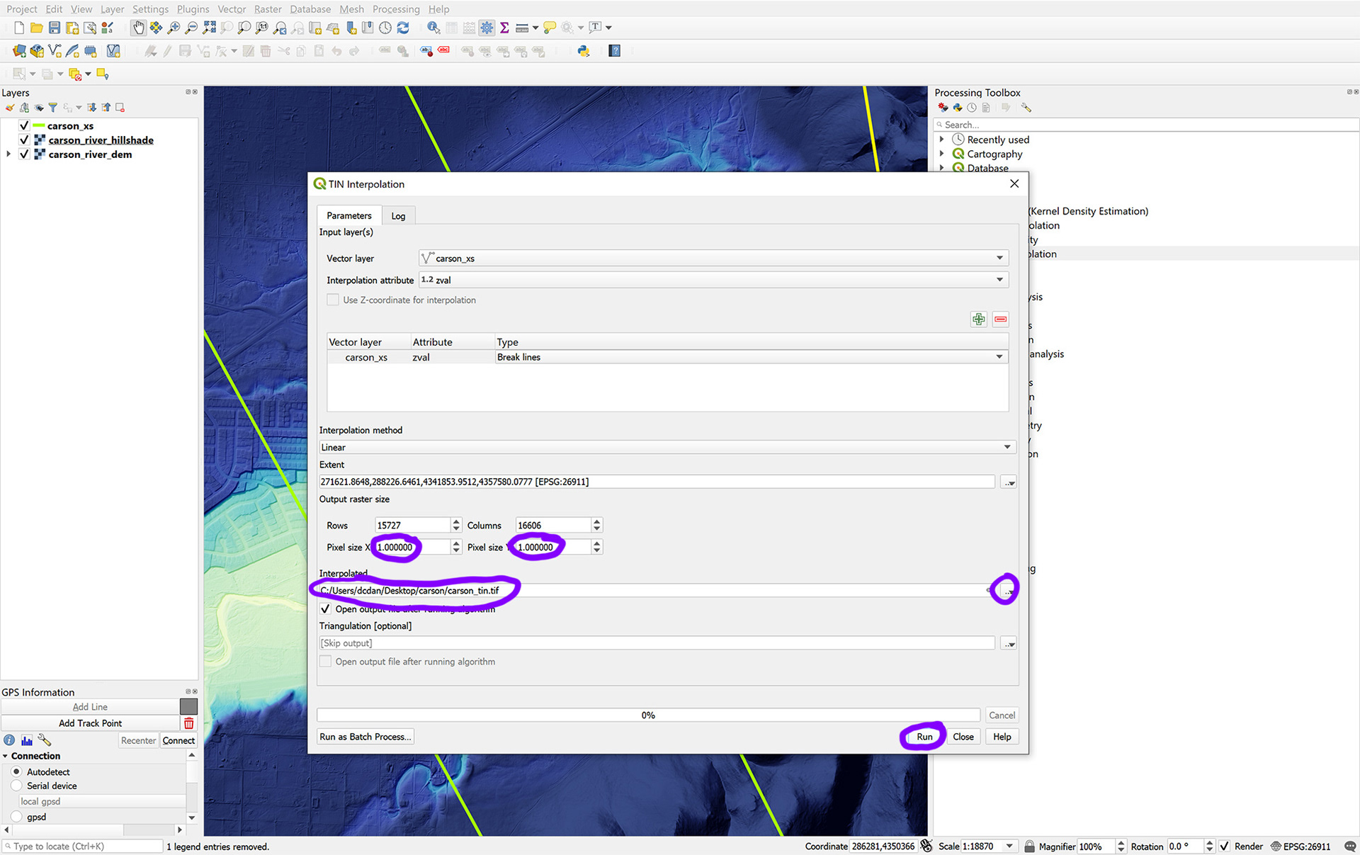
X. In the TIN Interpolation tool window select the cross section layer for the Vector layer.
For the Interpolation attribute select the zval attribute.
Click on the green plus button and then under the Type drop down menu, select Break Lines.
In the Extent drop down menu at right select Calculate from Layer and then your cross section layer.
Y. For the Pixel size enter the pixel size of your original DEM (in the example below the pixel size is 1 for our 1 meter DEM).
If you don't know the resolution of your DEM, you can find it in Layer Properties>Information>Pixel Size.
Under Interpolated, click the drop down menu at right (circled below) and select Save to File.
Then select the location and name of your file.
Then click Run.
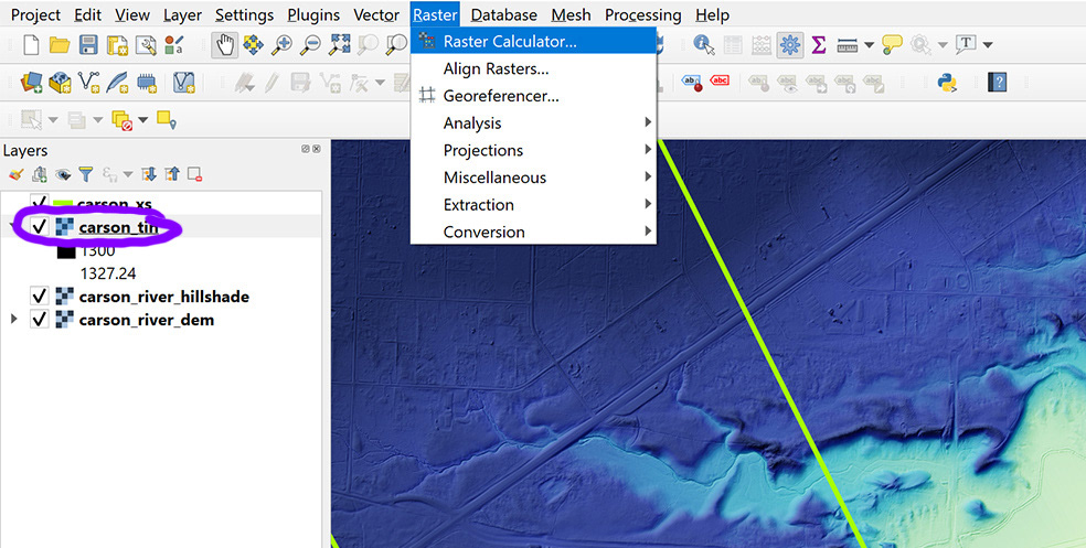
Z. When the Tin Interpolation tool is complete and the new file has been added to the Layer window, select Raster>Raster Calculator.
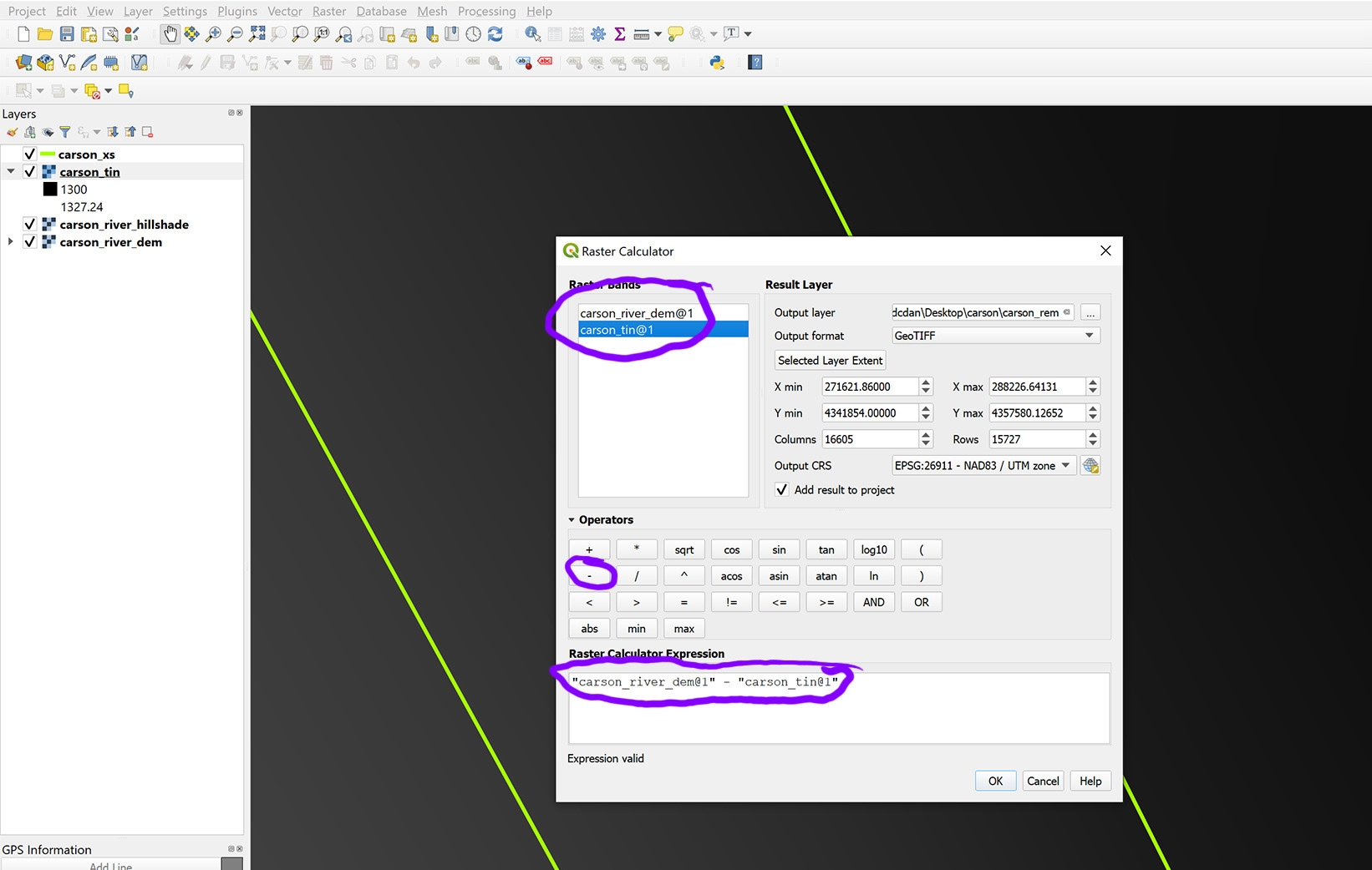
In the Raster Calculator window, select the file name and location next to Output layer (this will be your REM).
For Output format choose GeoTIFF.
Double click the DEM layer in the Raster Bands window to add it to the Raster Calculator Expression box below.
Then click on the minus sign to add a minus to the expression.
Finally, double click on the new TIN layer to add it to the expression and then click OK.
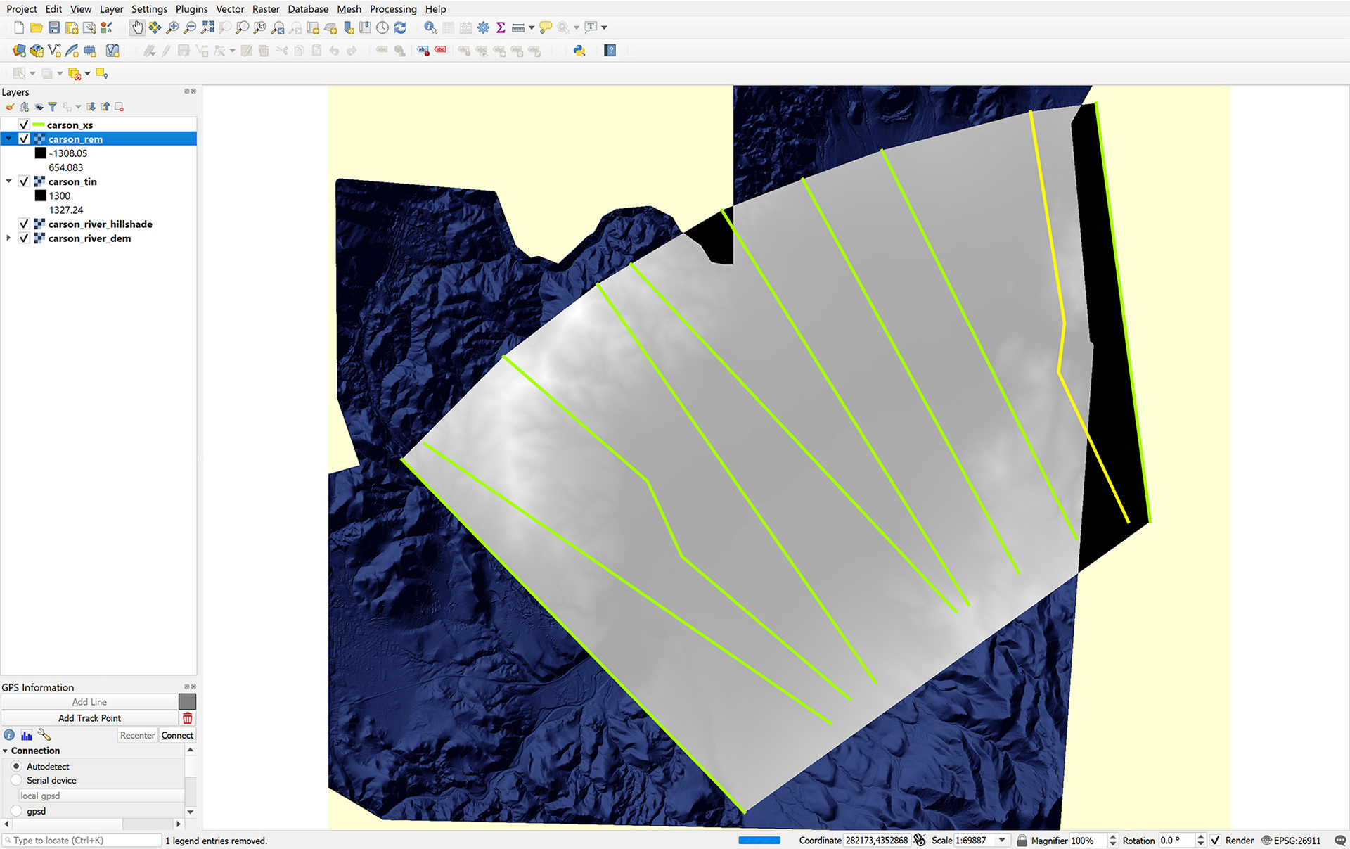
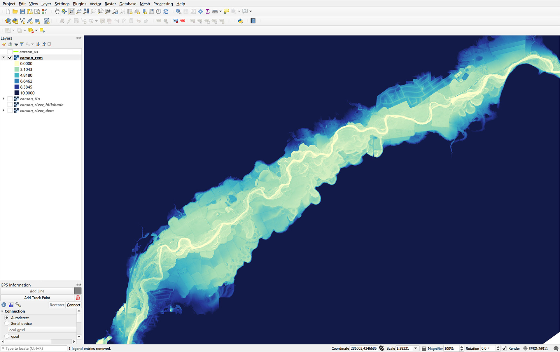
BB. When the process is complete the new REM file will be added to the Layers window and will look similar to the file below.
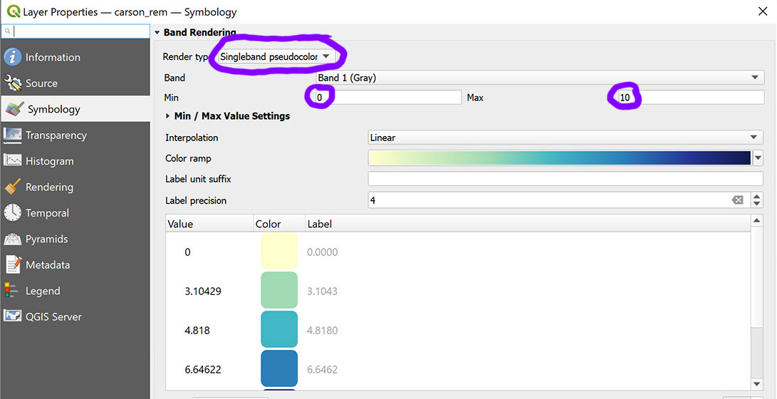
CC.In the Layer Properties window for the new REM file select Singleband pseudocolor for the Render type.
Enter 0 for the Min value and 10 for the Max value.
Then select the same color ramp as your original DEM. Select OK.
DD. Your REM will hopefully look something like the example below.
You can adjust the values—particularly the Max value—to get the desired visual result that you would like.
If there are unevenly-colored sections on the river surface (0 value end of the color ramp) you may need to go back and edit some of the cross section elevation values and re-run the tools/processes until you get smoother effect.
Remember that features like dams, steep waterfalls, tidal areas, braided channels, and mosaicked datasets from different time periods can can also introduce errors/anomalies in the visual appearance of REMs.
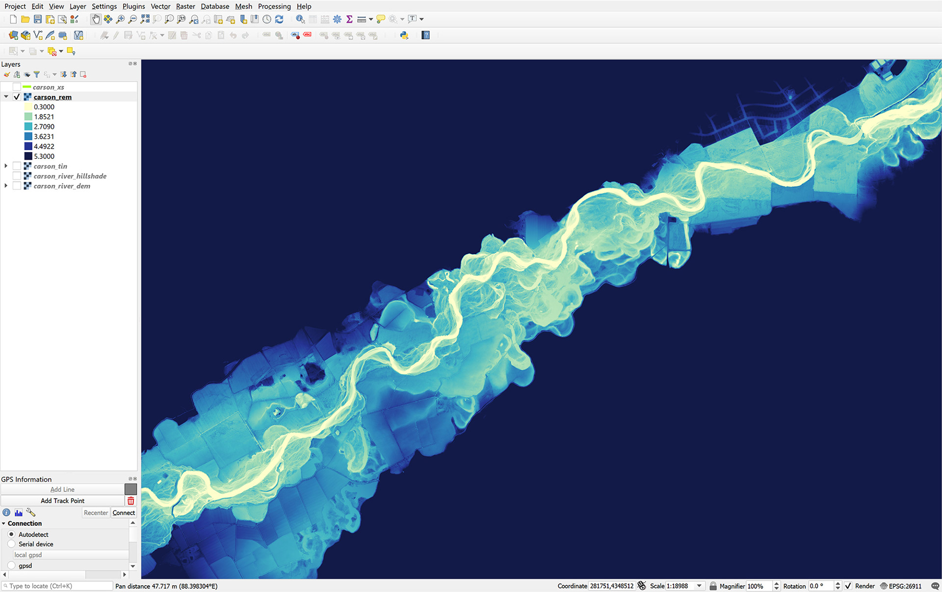
EE. Here is the same REM below (zoomed in a bit) with a 0 Min/5 Max value range.
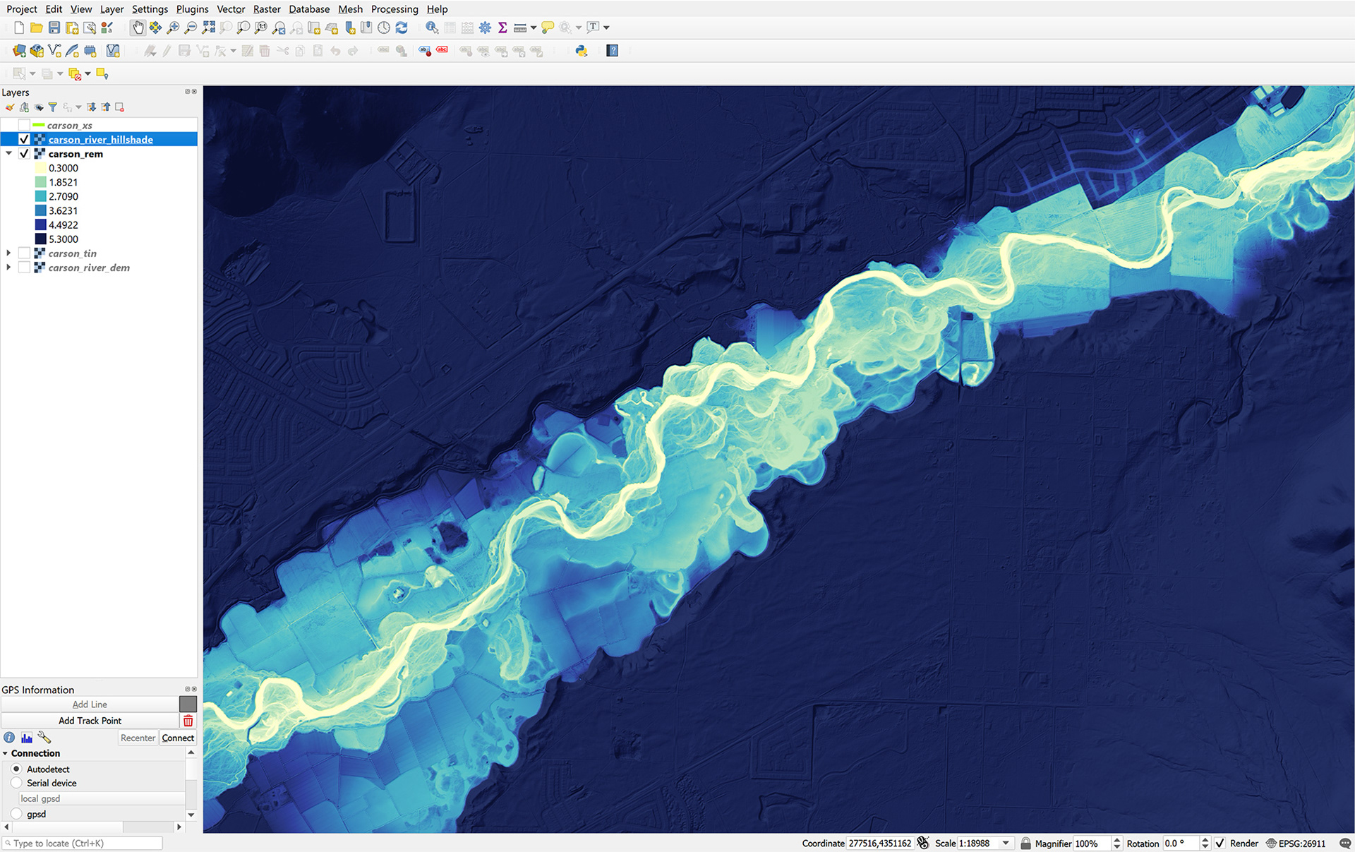
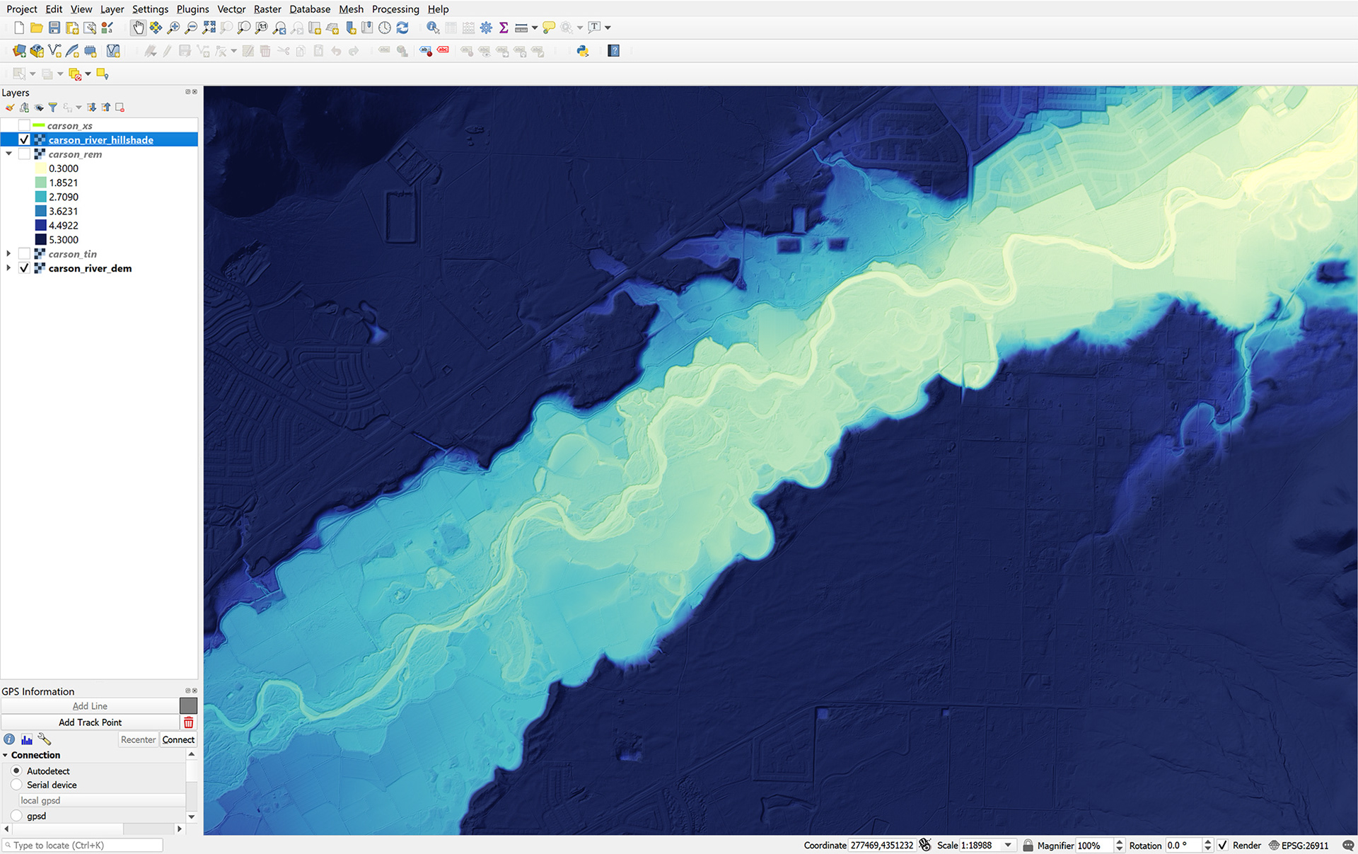
FF. And with the soft light hillshade overlaid on top of it.
GG. For a visual comparison, here is the original DEM below.
You can export the image from QGIS using the Layout function. Go to the Exporting Images from QGIS tutorial to learn more.
Congratulations on completing this tutorial! Hopefully you found this useful. If you have any questions, comments, or recommendations for making this better, use the contact page to send me a message. This is one of my first tutorials, so I look forward to fixing any mistakes that I made! I plan to add a video version of this and the other tutorials in the future.